Using SPIN
Gerard J. Holzmann
gerard@plan9.bell-labs.com
ABSTRACT
SPIN can be used for proving or disproving logical properties of concurrent systems. To render the proofs, a concurrent system is first modeled in a formal specification language called PROMELA. The language allows one to specify the behaviors of asynchronously executing processes that may interact through synchronous or asynchronous message passing, or through direct access to shared variables.
System models specified in this way can be verified for both safety and liveness properties. The specification of general properties in linear time temporal logic is also supported.
The first part of this manual discusses the basic features of the specification language PROMELA. The second part describes the verifier SPIN.
1. The Language PROMELA
PROMELA is short for Protocol Meta Language [Ho91]. PROMELA is a modeling language, not a programming language. A formal model differs in two essential ways from an implementation. First, a model is meant to be an abstraction of a design that contains only those aspects of the design that are directly relevant to the properties one is interested in proving. Second, a formal model must contain things that are typically not part of an implementation, such as worst-case assumptions about the behavior of the environment that may interact with the system being studied, and a formal statement of relevant correctness properties. It is possible to mechanically extract abstract models from implementation level code, as discussed, for instance in [HS99].
Verification with SPIN is often performed in a series of steps, with the construction of increasingly detailed models. Each model can be verified under different types of assumptions about the environment and for different types of correctness properties. If a property is not valid for the given assumptions about system behavior, the verifier can produce a counter-example that demonstrates how the property may be violated. If a property is valid, it may be possible to simplify the model based on that fact, and prove still other properties.
Section 1.1 covers the basic building blocks of the language. Section 1.2 introduces the control flow structures. Section 1.3 explains how correctness properties are specified. Section 1.4 concludes the first part with a discussion of special predefined variables and functions that can be used to express some correctness properties.
Up to date manual pages for SPIN can always be found online at: http://cm.bell-labs.com/cm/cs/what/spin/Man/
1.1. Basics
A PROMELA model can contain three different types of objects:
∙ Processes (section 1.1.1),
∙ Variables (section 1.1.2),
∙ Message channels (section 1.1.3).
All processes are global objects. For obvious reasons, a PROMELA model must contain at least one process to be meaningful. Since SPIN is specifically meant to prove properties of concurrent systems, a model typically contains more than one process.
Message channels and variables, the two basic types of data objects, can be declared with either a global scope or a local scope. A data object with global scope can be referred to by all processes. A data object with a local scope can be referred to by just a single process: the process that declares and instantiates the object. As usual, all objects must be declared in the specification before they are referenced.
1.1.1. Processes
Here is a simple process that does nothing except print a line of text:
init {
printf("it works\n")
}
There are a few things to note. Init is a predefined keyword from the language. It can be used to declare and instantiate a single initial process in the model. (It is comparable to the main procedure of a C program.) The init process does not take arguments, but it can start up (instantiate) other processes that do. Printf is one of a few built-in procedures in the language. It behaves the same as the C version. Note, finally, that no semicolon follows the single printf statement in the above example. In PROMELA, semicolons are used as statement separators, not statement terminators. (The SPIN parser, however, is lenient on this issue.)
Any process can start new processes by using another built-in procedure called run. For example,
proctype you_run(byte x)
{
printf("my x is: %d\n", x)
}
init {
run you_run(1);
run you_run(2)
}
The word proctype is again a keyword that introduces the declaration of a new type of process. In this case, we have named that type you_run and declared that all instantiations of processes of this type will take one argument: a data object of type byte, that can be referred to within this process by the name x. Instances of a proctype can be created with the predefined procedure run, as shown in the example. When the run statement completes, a copy of the process has been started, and all its arguments have been initialized with the arguments provided. The process may, but need not, have performed any statement executions at this point. It is now part of the concurrent system, and its execution can be interleaved arbitrarily with those of the other, already executing processes. (More about the semantics of execution follows shortly.)
In many cases, we are only interested in creating a single instance of each process type that is declared, and the processes require no arguments. We can define this by prefixing the keyword proctype from the process declaration with another keyword: active. Instances of all active proctypes are created when the system itself is initialized. We could, for instance, have avoided the use of init by declaring the corresponding process in the last example as follows:
active proctype main() {
run you_run(1);
run you_run(2)
}
Note that there are no parameters to instantiate in this case. Had they been declared, they would default to a zero value, just like all other data objects that are not explicitly instantiated.
Multiple copies of a process type can also be created in this way. For example:
active [4] proctype try_me() {
printf("hi, i am process %d\n", _pid)
}
creates four processes. A predefined variable _pid is assigned to each running process, and holds its unique process instantiation number. In some cases, this number is needed when a reference has to be made to a specific process.
Summarizing: process behavior is declared in proctype definitions, and it is instantiated with either run statements or with the prefix active. Within a proctype declaration, statements are separated (not terminated) by semicolons. As we shall see in examples that follow, instead of the semicolon, one can also use the alternative separator -> (arrow), wherever that may help to clarify the structure of a PROMELA model.
Semantics of Execution
In PROMELA there is no difference between a condition or expression and a statement. Fundamental to the semantics of the language is the notion of the executability of statements. Statements are either executable or blocked. Executability is the basic means of enforcing synchronization between the processes in a distributed system. A process can wait for an event to happen by waiting for a statement to become executable. For instance, instead of writing a busy wait loop:
while (a != b) /* not valid Promela syntax */
skip; /* wait for a==b */
...
we achieve the same effect in PROMELA with the statement
(a == b);
...
Often we indicate that the continuation of an execution is conditional on the truth of some expression by using the alternate statement separator:
(a == b) -> ...
Assignments and printf statements are always executable in PROMELA. A condition, however, can only be executed (passed) when it holds. If the condition does not hold, execution blocks until it does. There are similar rules for determining the executability of all other primitive and compound statements in the language. The semantics of each statement is defined in terms of rules for executability and effect. The rules for executability set a precondition on the state of the system in which a statement can be executed. The effect defines how a statement will alter a system state when executed.
PROMELA assumes that all individual statements are executed atomically: that is, they model the smallest meaningful entities of execution in the system being studied. This means that PROMELA defines the standard asynchronous interleaving model of execution, where a supposed scheduler is free at each point in the execution to select any one of the processes to proceed by executing a single primitive statement. Synchronization constraints can be used to influence the interleaving patterns. It is the purpose of a concurrent system’s design to constrain those patterns in such a way that no correctness requirements can be violated, and all service requirements are met. It is the purpose of the verifier either to find counter-examples to a designer’s claim that this goal has been met, or to demonstrate that the claim is indeed valid.
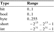
1.1.2. Variables
The table summarizes the five basic data types used in PROMELA. Bit and bool are synonyms for a single bit of information. The first three types can store only unsigned quantities. The last two can hold either positive or negative values. The precise value ranges of variables of types short and int is implementation dependent, and corresponds to those of the same types in C programs that are compiled for the same hardware. The values given in the table are most common.
The following example program declares a array of two elements of type bool and a scalar variable turn of the same type. Note that the example relies on the fact that _pid is either 0 or 1 here.
/*
* Peterson’s algorithm for enforcing
* mutual exclusion between two processes
* competing for access to a critical section
*/
bool turn, want[2];
active [2] proctype user()
{
again:
want[_pid] = 1; turn = _pid;
/* wait until this condition holds: */
(want[1 - _pid] == 0 || turn == 1 - _pid);
/* enter */
critical: skip;
/* leave */
want[_pid] = 0;
goto again
}
In the above case, all variables are initialized to zero. The general syntax for declaring and instantiating a variable, respectively for scalar and array variables, is:
type name = expression;
type name[constant] = expression
In the latter case, all elements of the array are initialized to the value of the expression. A missing initializer fields defaults to the value zero. As usual, multiple variables of the same type can be grouped behind a single type name, as in:
byte a, b[3], c = 4
In this example, the variable c is initialized to the value 4; variable a and the elements of array b are all initialized to zero.
Variables can also be declared as structures. For example:
typedef Field {
short f = 3;
byte g
};
typedef Msg {
byte a[3];
int fld1;
Field fld2;
chan p[3];
bit b
};
Msg foo;
introduces two user-defined data types, the first named Field and the second named Msg. A single variable named foo of type Msg is declared. All fields of foo that are not explicitly initialized (in the example, all fields except foo.fld2.f) are initialized to zero. References to the elements of a structure are written as:
foo.a[2] = foo.fld2.f + 12
A variable of a user-defined type can be passed as a single argument to a new process in run statements. For instance,
proctype me(Msg z) {
z.a[2] = 12
}
init {
Msg foo;
run me(foo)
}
Note that even though PROMELA supports only one-dimensional arrays, a two-dimensional array can be created indirectly with user-defined structures, for instance as follows:
typedef Array {
byte el[4]
};
Array a[4];
This creates a data structure of 16 elements that can be referenced, for instance, as a[i].el[j].
As in C, the indices of an array of N elements range from 0 to N-1.
Expressions
Expressions must be side-effect free in PROMELA. Specifically, this means that an expression cannot contain assignments, or send and receive operations (see section 1.1.3).
c = c + 1; c = c - 1
and
c++; c--
are assignments in PROMELA, with the same effects. But, unlike in C,
b = c++
is not a valid assignment, because the right-hand side operand is not a valid expression in PROMELA (it is not side-effect free).
It is also possible to write a side-effect free conditional expression, with the following syntax:
(expr1 -> expr2 : expr3)
The parentheses around the conditional expression are required to avoid misinterpretation of the arrow. The example expression has the value of expr2 when expr1 evaluates to a non-zero value, and the value of expr3 otherwise.
In assignments like
variable = expression
the values of all operands used inside the expression are first cast to signed integers before the operands are applied. After the evaluation of the expression completes, the value produced is cast to the type of the target variable before the assignment takes place.
1.1.3. Message Channels
Message channels are used to model the transfer of data between processes. They are declared either locally or globally, for instance as follows:
chan qname = [16] of { short, byte }
The keyword chan introduces a channel declaration. In this case, the channel is named qname, and it is declared to be capable of storing up to 16 messages. Each message stored in the channel is declared here to consist of two fields: one of type short and one of type byte. The fields of a message can be any one of the basic types bit, bool, byte, short, int, and chan, or any user-defined type. Message fields cannot be declared as arrays.
A message field of type chan can be used to pass a channel identifier through a channel from one process to another.
The statement
qname!expr1,expr2
sends the values of expressions expr1 and expr2 to the channel that we just created. It appends the message field created from the values of the two expressions (and cast to the appropriate types of the message fields declared for qname) to the tail of the message buffer of 16 slots that belongs to channel qname. By default the send statement is only executable if the target channel is non-full. (This default semantics can be changed in the verifier into one where the send statement is always executable, but the message will be lost when an attempt is made to append it to a full channel.)
The statement
qname?var1,var2
retrieves a message from the head of the same buffer, and stores the two expressions in variables var1 and var2.
The receive statement is executable only if the source channel is non-empty.
If more parameters are sent per message than were declared for the message channel, the redundant parameters are lost. If fewer parameters are sent than declared, the value of the remaining parameters is undefined. Similarly, if the receive operation tries to retrieve more parameters than available, the value of the extra parameters is undefined; if it receives fewer than the number of parameters sent, the extra information is lost.
An alternative, and equivalent, notation for the send and receive operations is to structure the message fields with parentheses, as follows:
qname!expr1(expr2,expr3)
qname?var1(var2,var3)
In the above case, we assume that qname was declared to hold messages consisting of three fields.
Some or all of the arguments of the receive operation can be given as constants instead of as variables:
qname?cons1,var2,cons2
In this case, an extra condition on the executability of the receive operation is that the value of all message fields specified as constants match the value of the corresponding fields in the message that is to be received.
Here is an example that uses some of the mechanisms introduced so far.
proctype A(chan q1)
{ chan q2;
q1?q2;
q2!123
}
proctype B(chan qforb)
{ int x;
qforb?x;
printf("x = %d\n", x)
}
init {
chan qname = [1] of { chan };
chan qforb = [1] of { int };
run A(qname);
run B(qforb);
qname!qforb
}
The value printed by the process of type B will be 123.
A predefined function len(qname) returns the number of messages currently stored in channel qname. Two shorthands for the most common uses of this function are empty(qname) and full(qname), with the obvious connotations.
Since all expressions must be side-effect free, it is not valid to say:
(qname?var == 0)
or
(a > b && qname!123)
We could rewrite the second example (using an atomic sequence, as explained further in section 1.2.1):
atomic { (a > b && !full(qname)) -> qname!123 }
The meaning of the first example is ambiguous. It could mean that we want the condition to be true if the receive operation is unexecutable. In that case, we can rewrite it without side-effects as:
empty(qname)
It could also mean that we want the condition to be true when the channel does contain a message with value zero. We can specify that as follows:
atomic { qname?[0] -> qname?var }
The first statement of this atomic sequence is an expression without side-effects that evaluates to a non-zero value only if the receive operation
qname?0
would have been executable at that point (i.e., channel qname contains at least one message and the oldest message stored consists of one message field equal to zero). Any receive statement can be turned into a side-effect free expression by placing square brackets around the list of all message parameters. The channel contents remain undisturbed by the evaluation of such expressions.
Note carefully, however, that in non-atomic sequences of two statements such as
!full(qname) -> qname!msgtype
and
qname?[msgtype] -> qname?msgtype
the second statement is not necessarily executable after the first one has been executed. There may be race conditions when access to the channels is shared between several processes. Another process can send a message to the channel just after this process determined that it was not full, or another process can steal away the message just after our process determined its presence.
Two other types of send and receive statements are used less frequently: sorted send and random receive. A sorted send operation is written with two, instead of one, exclamation marks, as follows:
qname!!msg
A sorted send operation will insert a message into the channel’s buffer in numerical order, instead of in FIFO order. The channel contents are scanned from the first message towards the last, and the message is inserted immediately before the first message that follows it in numerical order. To determine the numerical order, all message fields are taken into account.
The logical counterpart of the sorted send operation is the random receive. It is written with two, instead of one, question marks:
qname??msg
A random receive operation is executable if it is executable for any message that is currently buffered in a message channel (instead of only for the first message in the channel). Normal send and receive operations can freely be combined with sorted send and random receive operations.
Rendezvous Communication
So far we have talked about asynchronous communication between processes via message channels, declared in statements such as
chan qname = [N] of { byte }
where N is a positive constant that defines the buffer size. A logical extension is to allow for the declaration
chan port = [0] of { byte }
to define a rendezvous port. The channel size is zero, that is, the channel port can pass, but cannot store, messages. Message interactions via such rendezvous ports are by definition synchronous. Consider the following example:
#define msgtype 33
chan name = [0] of { byte, byte };
active proctype A()
{ name!msgtype(124);
name!msgtype(121)
}
active proctype B()
{ byte state;
name?msgtype(state)
}
Channel name is a global rendezvous port. The two processes will synchronously execute their first statement: a handshake on message msgtype and a transfer of the value 124 to local variable state. The second statement in process A will be unexecutable, because there is no matching receive operation in process B.
If the channel name is defined with a non-zero buffer capacity, the behavior is different. If the buffer size is at least 2, the process of type A can complete its execution, before its peer even starts. If the buffer size is 1, the sequence of events is as follows. The process of type A can complete its first send action, but it blocks on the second, because the channel is now filled to capacity. The process of type B can then retrieve the first message and complete. At this point A becomes executable again and completes, leaving its last message as a residual in the channel.
Rendezvous communication is binary: only two processes, a sender and a receiver, can be synchronized in a rendezvous handshake.
As the example shows, symbolic constants can be defined with preprocessor macros using #define. The source text of a PROMELA model is translated by the standard C preprocessor. The disadvantage of defining symbolic names in this way is, however, that the PROMELA parser will only see the expanded text, and cannot refer to the symbolic names themselves. To prevent that, PROMELA also supports another way to define symbolic names, which are preserved in error reports. For instance, by including the declaration
mtype = { ack, msg, error, data };
at the top of a PROMELA model, the names provided between the curly braces are equivalent to integers of type byte, but known by their symbolic names to the SPIN parser and the verifiers it generates. The constant values assigned start at 1, and count up. There can be only one mtype declaration per model.
1.2. Control Flow
So far, we have seen only some of the basic statements of PROMELA, and the way in which they can be combined to model process behaviors. The five types of statements we have mentioned are: printf, assignment, condition, send, and receive.
The pseudo-statement skip is syntactically and semantically equivalent to the condition (1) (i.e., to true), and is in fact quietly replaced with this expression by the lexical analyzer of SPIN.
There are also five types of compound statements.
∙ Atomic sequences (section 1.2.1),
∙ Deterministic steps (section 1.2.2),
∙ Selections (section 1.2.3),
∙ Repetitions (section 1.2.4),
∙ Escape sequences (section 1.2.5).
1.2.1. Atomic Sequences
The simplest compound statement is the atomic sequence:
atomic { /* swap the values of a and b */
tmp = b;
b = a;
a = tmp
}
In the example, the values of two variables a and b are swapped in a sequence of statement executions that is defined to be uninterruptable. That is, in the interleaving of process executions, no other process can execute statements from the moment that the first statement of this sequence begins to execute until the last one has completed.
It is often useful to use atomic sequences to start a series of processes in such a way that none of them can start executing statements until all of them have been initialized:
init {
atomic {
run A(1,2);
run B(2,3);
run C(3,1)
}
}
Atomic sequences may be non-deterministic. If any statement inside an atomic sequence is found to be unexecutable, however, the atomic chain is broken, and another process can take over control. When the blocking statement becomes executable later, control can non-deterministically return to the process, and the atomic execution of the sequence resumes as if it had not been interrupted.
1.2.2. Deterministic Steps
Another way to define an indivisible sequence of actions is to use the d_step statement. In the above case, for instance, we could also have written:
d_step { /* swap the values of a and b */
tmp = b;
b = a;
a = tmp
}
The difference between a d_step sequence and an atomic sequence are:
∙ A d_step sequence must be completely deterministic. (If non-determinism is nonetheless encountered, it is always resolved in a fixed and deterministic way: i.e., the first true guard in selection or repetition structures is always selected.)
∙ No goto jumps into or out of a d_step sequence are permitted.
∙ The execution of a d_step sequence cannot be interrupted when a blocking statement is encountered. It is an error if any statement other than the first one in a d_step sequence is found to be unexecutable.
∙ A d_step sequence is executed as one single statement. In a way, it is a mechanism for adding new types of statements to the language.
None of the items listed above apply to atomic sequences. This means that the keyword d_step can always be replaced with the keyword atomic, but the reverse is not true. (The main, perhaps the only, reason for using d_step sequences is to improve the efficiency of verifications.)
1.2.3. Selection Structures
A more interesting construct is the selection structure. Using the relative values of two variables a and b to choose between two options, for instance, we can write:
if
:: (a != b) -> option1
:: (a == b) -> option2
fi
The selection structure above contains two execution sequences, each preceded by a double colon. Only one sequence from the list will be executed. A sequence can be selected only if its first statement is executable. The first statement is therefore called a guard.
In the above example the guards are mutually exclusive, but they need not be. If more than one guard is executable, one of the corresponding sequences is selected nondeterministically. If all guards are unexecutable the process will block until at least one of them can be selected. There is no restriction on the type of statements that can be used as a guard: it may include sends or receives, assignments, printf, skip, etc. The rules of executability determine in each case what the semantics of the complete selection structure will be. The following example, for instance, uses receive statements as guards in a selection.
mtype = { a, b };
chan ch = [1] of { byte };
active proctype A()
{ ch!a
}
active proctype B()
{ ch!b
}
active proctype C()
{ if
:: ch?a
:: ch?b
fi
}
The example defines three processes and one channel. The first option in the selection structure of the process of type C is executable if the channel contains a message named a, where a is a symbolic constant defined in the mtype declaration at the start of the program. The second option is executable if it contains a message b, where, similarly, b is a symbolic constant. Which message will be available depends on the unknown relative speeds of the processes.
A process of the following type will either increment or decrement the value of variable count once.
byte count;
active proctype counter()
{
if
:: count++
:: count--
fi
}
Assignments are always executable, so the choice made here is truly a non-deterministic one that is independent of the initial value of the variable (zero in this case).
1.2.4. Repetition Structures
We can modify the above program as follows, to obtain a cyclic program that randomly changes the value of the variable up or down, by replacing the selection structure with a repetition.
byte count;
active proctype counter()
{
do
:: count++
:: count--
:: (count == 0) -> break
od
}
Only one option can be selected for execution at a time. After the option completes, the execution of the structure is repeated. The normal way to terminate the repetition structure is with a break statement. In the example, the loop can be broken only when the count reaches zero. Note, however, that it need not terminate since the other two options remain executable. To force termination we could modify the program as follows.
active proctype counter()
{
do
:: (count != 0) ->
if
:: count++
:: count--
fi
:: (count == 0) -> break
od
}
A special type of statement that is useful in selection and repetition structures is the else statement. An else statement becomes executable only if no other statement within the same process, at the same control-flow point, is executable. We could try to use it in two places in the above example:
active proctype counter()
{
do
:: (count != 0) ->
if
:: count++
:: count--
:: else
fi
:: else -> break
od
}
The first else, inside the nested selection structure, can never become executable though, and is therefore redundant (both alternative guards of the selection are assignments, which are always executable). The second usage of the else, however, becomes executable exactly when !(count != 0) or (count == 0), and is therefore equivalent to the latter to break from the loop.
There is also an alternative way to exit the do-loop, without using a break statement: the infamous goto. This is illustrated in the following implementation of Euclid’s algorithm for finding the greatest common divisor of two non-zero, positive numbers:
proctype Euclid(int x, y)
{
do
:: (x > y) -> x = x - y
:: (x < y) -> y = y - x
:: (x == y) -> goto done
od;
done:
skip
}
init { run Euclid(36, 12) }
The goto in this example jumps to a label named done. Since a label can only appear before a statement, we have added the dummy statement skip. Like a skip, a goto statement is always executable and has no other effect than to change the control-flow point of the process that executes it.
As a final example, consider the following implementation of a Dijkstra semaphore, which is implemented with the help of a synchronous channel.
#define p 0
#define v 1
chan sema = [0] of { bit };
active proctype Dijkstra()
{ byte count = 1;
do
:: (count == 1) ->
sema!p; count = 0
:: (count == 0) ->
sema?v; count = 1
od
}
active [3] proctype user()
{ do
:: sema?p;
/* critical section */
sema!v;
/* non-critical section */
od
}
The semaphore guarantees that only one of the three user processes can enter its critical section at a time. It does not necessarily prevent the monopolization of the access to the critical section by one of the processes.
PROMELA does not have a mechanism for defining functions or procedures. Where necessary, though, these may be modeled with the help of additional processes. The return value of a function, for instance, can be passed back to the calling process via global variables or messages. The following program illustrates this by recursively calculating the factorial of a number n.
proctype fact(int n; chan p)
{ chan child = [1] of { int };
int result;
if
:: (n <= 1) -> p!1
:: (n >= 2) ->
run fact(n-1, child);
child?result;
p!n*result
fi
}
init
{ chan child = [1] of { int };
int result;
run fact(7, child);
child?result;
printf("result: %d\n", result)
}
Each process creates a private channel and uses it to communicate with its direct descendant. There are no input statements in PROMELA. The reason is that models must always be complete to allow for logical verifications, and input statements would leave at least the source of some information unspecified. A way to read input would presuppose a source of information that is not part of the model.
We have already discussed a few special types of statement: skip, break, and else. Another statement in this class is the timeout. The timeout is comparable to a system level else statement: it becomes executable if and only if no other statement in any of the processes is executable. Timeout is a modeling feature that provides for an escape from a potential deadlock state. The timeout takes no parameters, because the types of properties we would like to prove for PROMELA models must be proven independent of all absolute and relative timing considerations. In particular, the relative speeds of processes can never be known with certainty in an asynchronous system.
1.2.5. Escape Sequences
The last type of compound structure to be discussed is the unless statement. It is used as follows:
{ P } unless { E }
where the letters P and E represent arbitrary PROMELA fragments. Execution of the unless statement begins with the execution of statements from P. Before each statement execution in P the executability of the first statement of E is checked, using the normal PROMELA semantics of executability. Execution of statements from P proceeds only while the first statement of E remains unexecutable. The first time that this ‘guard of the escape sequence’ is found to be executable, control changes to it, and execution continues as defined for E. Individual statement executions remain indivisible, so control can only change from inside P to the start of E in between individual statement executions. If the guard of the escape sequence does not become executable during the execution of P, then it is skipped entirely when P terminates.
An example of the use of escape sequences is:
A;
do
:: b1 -> B1
:: b2 -> B2
...
od
unless { c -> C };
D
As shown in the example, the curly braces around the main sequence (or the escape sequence) can be deleted if there can be no confusion about which statements belong to those sequences. In the example, condition c acts as a watchdog on the repetition construct from the main sequence. Note that this is not necessarily equivalent to the construct
A;
do
:: b1 -> B1
:: b2 -> B2
...
:: c -> break
od;
C; D
if B1 or B2 are non-empty. In the first version of the example, execution of the iteration can be interrupted at any point inside each option sequence. In the second version, execution can only be interrupted at the start of the option sequences.
1.3. Correctness Properties
There are three ways to express correctness properties in PROMELA, using:
∙ Assertions (section 1.3.1),
∙ Special labels (section 1.3.2),
∙ Never claims (section 1.3.3).
1.3.1. Assertions
Statements of the form
assert(expression)
are always executable. If the expression evaluates to a non-zero value (i.e., the corresponding condition holds), the statement has no effect when executed. The correctness property expressed, though, is that it is impossible for the expression to evaluate to zero (i.e., for the condition to be false). A failing assertion will cause execution to be aborted.
1.3.2. Special Labels
Labels in a PROMELA specification ordinarily serve as targets for unconditional goto jumps, as usual. There are, however, also three types of labels that have a special meaning to the verifier. We discuss them in the next three subsections.
1.3.2.1. End-State Labels
When a PROMELA model is checked for reachable deadlock states by the verifier, it must be able to distinguish valid end states from invalid ones. By default, the only valid end states are those in which every PROMELA process that was instantiated has reached the end of its code. Not all PROMELA processes, however, are meant to reach the end of their code. Some may very well linger in a known wait state, or they may sit patiently in a loop ready to spring into action when new input arrives.
To make it clear to the verifier that these alternate end states are also valid, we can define special end-state labels. We can do so, for instance, in the process type Dijkstra, from an earlier example:
proctype Dijkstra()
{ byte count = 1;
end: do
:: (count == 1) ->
sema!p; count = 0
:: (count == 0) ->
sema?v; count = 1
od
}
The label end defines that it is not an error if, at the end of an execution sequence, a process of this type has not reached its closing curly brace, but waits at the label. Of course, such a state could still be part of a deadlock state, but if so, it is not caused by this particular process.
There may be more than one end-state label per PROMELA model. If so, all labels that occur within the same process body must be unique. The rule is that every label name with the prefix end is taken to be an end-state label.
1.3.2.2. Progress-State Labels
In the same spirit, PROMELA also allows for the definition of progress labels. Passing a progress label during an execution is interpreted as a good thing: the process is not just idling while waiting for things to happen elsewhere, but is making effective progress in its execution. The implicit correctness property expressed here is that any infinite execution cycle allowed by the model that does not pass through at least one of these progress labels is a potential starvation loop. In the Dijkstra example, for instance, we can label the successful passing of a semaphore test as progress and ask a verifier to make sure that there is no cycle elsewhere in the system.
proctype Dijkstra()
{ byte count = 1;
end: do
:: (count == 1) ->
progress: sema!p; count = 0
:: (count == 0) ->
sema?v; count = 1
od
}
If more than one state carries a progress label, variations with a common prefix are again valid.
1.3.2.3. Accept-State Labels
The last type of label, the accept-state label, is used primarily in combination with never claims. Briefly, by labeling a state with any label starting with the prefix accept we can ask the verifier to find all cycles that do pass through at least one of those labels. The implicit correctness claim is that this cannot happen. The primary place where accept labels are used is inside never claims. We discuss never claims next.
1.3.3. Never Claims
Up to this point we have talked about the specification of correctness criteria with assertions and with three special types of labels. Powerful types of correctness criteria can already be expressed with these tools, yet so far our only option is to add them to individual proctype declarations. We can, for instance, express the claim ‘‘every system state in which property P is true eventually leads to a system state in which property Q is true,’’ with an extra monitor process, such as:
active proctype monitor()
{
progress:
do
:: P -> Q
od
}
If we require that property P must remain true while we are waiting Q to become true, we can try to change this to:
active proctype monitor()
{
progress:
do
:: P -> assert(P || Q)
od
}
but this does not quite do the job. Note that we cannot make any assumptions about the relative execution speeds of processes in a PROMELA model. This means that if in the remainder of the system the property P becomes true, we can move to the state just before the assert, and wait there for an unknown amount of time (anything between a zero delay and an infinite delay is possible here, since no other synchronizations apply). If Q becomes true, we may pass the assertion, but we need not do so. Even if P becomes false only after Q has become true, we may still fail the assertion, as long as there exists some later state where neither P nor Q is true. This is clearly unsatisfactory, and we need another mechanism to express these important types of liveness properties.
The Connection with Temporal Logic
A general way to express system properties of the type we have just discussed is to use linear time temporal logic (LTL) formulae. Every PROMELA expression is automatically also a valid LTL formula. An LTL formula can also contain the unary temporal operators □ (pronounced always), ◊ (pronounced eventually), and two binary temporal operators U (pronounced weak until) and U (pronounced strong until).
Where the value of a PROMELA expression without temporal operators can be defined uniquely for individual system states, without further context, the truth value of an LTL formula is defined for sequences of states: specifically, it is defined for the first state of a given infinite sequence of system states (a trace). Given, for instance, the sequence of system states:
s0;s1;s2;...
the LTL formula pUq, with p and q standard PROMELA expressions, is true for s0 either if q is true in s0, or if p is true in s0 and pUq holds for the remainder of the sequence after s0.
Informally, pUq says that p is required to hold at least until q becomes true. If, instead, we would write pUq, then we also require that there exists at least one state in the sequence where q does indeed become true.
The temporal operators □ and ◊ can be defined in terms of the strong until operator U, as follows.
□ p = !◊ !p = !(true U !p)
Informally, □ p says that property p must hold in all states of a trace, and ◊ p says that p holds in at least one state of the trace.
To express our original example requirement: ‘‘every system state in which property P is true eventually leads to a system state in which property Q is true,’’ we can write the LTL formula:
□ (P -> ◊ Q)
where the logical implication symbol -> is defined in the usual way as
P => Q means !P || Q
Mapping LTL Formulae onto Never Claims
PROMELA does not include syntax for specifying LTL formulae directly, but it relies on the fact that every such formula can be translated into a special type of automaton, known as a Büchi automaton. In the syntax of PROMELA this automaton is called a never claim. If you don’t care too much about the details of never claims, you can skip the remainder of this section and simple remember that SPIN can convert any LTL formula automatically into the proper never claim syntax with the command:
spin -f "...formula..."
Here are the details. The syntax of a never claim is:
never {
...
}
where the dots can contain any PROMELA fragment, including arbitrary repetition, selection, unless constructs, jumps, etc.
There is an important difference in semantics between a proctype declaration and a never claim. Every statement inside a never claim is interpreted as a proposition, i.e., a condition. A never claim should therefore only contain expressions and never statements that can have side-effects (assignments, sends or receives, run-statements, etc.)
Never claims are used to express behaviors that are considered undesirable or illegal. We say that a never claim is ‘matched’ if the undesirable behavior can be realized, contrary to the claim, and thus the correctness requirement violated. The claims are evaluated over system executions, that is, the propositions that are listed in the claim are evaluated over the traces from the remainder of the system. The claim, therefore, should not alter that behavior: it merely monitors it. Every time that the system reaches a new state, by asynchronously executing statements from the model, the claim will evaluate the appropriate propositions to determine if a counter-example can be constructed to the implicit LTL formula that is specified.
Since LTL formulae are only defined for infinite executions, the behavior of a never claim can only be matched by an infinite system execution. This by itself would restrict us to the use of progress labels and accept labels as the only means we have discussed so far for expressing properties of infinite behaviors. To conform to standard omega automata theory, the behaviors of never claims are expressed exclusively with accept labels (never with progress labels). To match a claim, therefore, an infinite sequence of true propositions must exist, at least one of which is labeled with an accept label (inside the never claim).
Since PROMELA models can also express terminating system behaviors, we have to define the semantics of the never claims also for those behaviors. To facilitate this, it is defined that a never claim can also be matched when it reaches its closing curly brace (i.e., when it appears to terminate). This semantics is based on what is usually referred to as a ‘stuttering semantics.’ With stuttering semantics, any terminating execution can be extended into an equivalent infinite execution (for the purposes of evaluating LTL properties) by repeating (stuttering) the final state infinitely often. As a syntactical convenience, the final state of a never claim is defined to be accepting, i.e., it could be replaced with the explicit repetition construct:
accept: do :: skip od
Every process behavior, similarly, is (for the purposes of evaluating the never claims) thought to be extended with a dummy self-loop on all final states:
do :: skip od
(Note the accept labels only occur in the never claim, not in the system.)
The Semantics of a Never Claim
Never claims are probably the hardest part of the language to understand, so it is worth spending a few extra words on them. On an initial reading, feel free to skip the remainder of this section.
The difference between a never claim and the remainder of a PROMELA system can be explained as follows. A PROMELA model defines an asynchronous interleaving product of the behaviors of individual processes. Given an arbitrary system state, its successor states are conceptually obtained in two steps. In a first step, all the executable statements in the individual processes are identified. In a second step, each one of these statements is executed, each one producing one potential successor for the current state. The complete system behavior is thus defined recursively and represents all possible interleavings of the individual process behaviors. It is this asynchronous product machine that we call the ‘global system behavior’.
The addition of a never claim defines a synchronous product of the global system behavior with the behavior expressed in the claim. This synchronous product can be thought of as the construction of a new global state machine, in which every state is defined as a pair (s,n) with s a state from the global system (the asynchronous product of processes), and n a state from the claim. Every transition in the new global machine is similarly defined by a pair of transitions, with the first element a statement from the system, and the second a proposition from the claim. In other words, every transition in this final synchronous product is defined as a joint transition of the system and the claim. Of course, that transition can only occur if the proposition from the second half of the transition pair evaluates to true in the current state of the system (the first half of the state pair).
Examples
To manually translate an LTL formula into a never claim (e.g. foregoing the builtin translation that SPIN offers), we must carefully consider whether the formula expresses a positive or a negative property. A positive property expresses a good behavior that we would like our system to have. A negative property expresses a bad behavior that we claim the system does not have. A never claim can express only negative claims, not positive ones. Fortunately, the two are exchangeable: if we want to express that a good behavior is unavoidable, we can formalize all ways in which the good behavior could be violated, and express that in the never claim.
Suppose that the LTL formula ◊□ p, with p a PROMELA expression, expresses a negative claim (i.e., it is considered a correctness violation if there exists any execution sequence in which p can eventually remain true infinitely long). This can be written in a never claim as:
never { /* <>[]p */
do
:: skip /* after an arbitrarily long prefix */
:: p -> break /* p becomes true */
od;
accept: do
:: p /* and remains true forever after */
od
}
Note that in this case the claim does not terminate, and also does not necessarily match all system behaviors. It is sufficient if it precisely captures all violations of our correctness requirement, and no more.
If the LTL formula expressed a positive property, we first have to invert it to the corresponding negative property ◊!p and translate that into a never claim. The requirement now says that it is a violation if p does not hold infinitely long.
never { /* <>!p*/
do
:: skip
:: !p -> break
od
}
We have used the implicit match of a claim upon reaching the closing terminating brace. Since the first violation of the property suffices to disprove it, we could also have written:
never { /* <>!p*/
do
:: p
:: !p -> break
od
}
or, if we abandon the connection with LTL for a moment, even more tersely as:
never { do :: assert(p) od }
Suppose we wish to express that it is a violation of our correctness requirements if there exists any execution in the system where □ (p -> ◊ q) is violated (i.e., the negation of this formula is satisfied). The following never claim expresses that property:
never {
do
:: skip
:: p && !q -> break
od;
accept:
do
:: !q
od
}
Note that using (!p || q) instead of skip in the first repetition construct would imply a check for just the first occurrence of proposition p becoming true in the execution sequence, while q is false. The above formalization checks for all occurrences, anywhere in a trace.
Finally, consider a formalization of the LTL property □ (p -> (q U r)). The corresponding claim is:
never {
do
:: skip /* to match any occurrence */
:: p && q && !r -> break
:: p && !q && !r -> goto error
od;
do
:: q && !r
:: !q && !r -> break
od;
error: skip
}
Note again the use of skip instead of (!p || r) to avoid matching just the first occurrence of (p && !r) in a trace.
1.4. Predefined Variables and Functions
The following predefined variables and functions can be especially useful in never claims.
The predefined variables are: _pid and _last.
_pid is a predefined local variable in each process that holds the unique instantiation number for that process. It is always a non-negative number.
_last is a predefined global variable that always holds the instantiation number of the process that performed the last step in the current execution sequence. Its value is not part of the system state unless it is explicitly used in a specification.
never {
/* it is not possible for the process with pid=1
* to execute precisely every other step forever
*/
accept:
do
:: _last != 1 -> _last == 1
od
}
The initial value of _last is zero.
Three predefined functions are specifically intended to be used in never claims, and may not be used elsewhere in a model: pc_value(pid), enabled(pid), procname[pid]@label.
The function pc_value(pid) returns the current control state of the process with instantiation number pid, or zero if no such process exists.
Example:
never {
/* Whimsical use: claim that it is impossible
* for process 1 to remain in the same control
* state as process 2, or one with smaller value.
*/
accept: do
:: pc_value(1) <= pc_value(2)
od
}
The function enabled(pid) tells whether the process with instantiation number pid has an executable statement that it can execute next.
Example:
never {
/* it is not possible for the process with pid=1
* to remain enabled without ever executing
*/
accept:
do
:: _last != 1 && enabled(1)
od
}
The last function procname[pid]@label tells whether the process with instantiation number pid is currently in the state labeled with label in proctype procname. It is an error if the process referred to is not an instantiation of that proctype.
2. Verifications with SPIN
The easiest way to use SPIN is probably on a Windows terminal with the Tcl/Tk implementation of XSPIN. All functionality of SPIN, however, is accessible from any plain ASCII terminal, and there is something to be said for directly interacting with the tool itself.
The description in this paper gives a short walk-through of a common mode of operation in using the verifier. A more tutorial style description of the verification process can be found in [Ho93]. More detail on the verification of large systems with the help of SPIN’s supertrace (bitstate) verification algorithm can be found in [Ho95].
∙ Random and interactive simulations (section 2.1),
∙ Generating a verifier (section 2.2),
∙ Compilation for different types of searches (section 2.3),
∙ Performing the verification (section 2.4),
∙ Inspecting error traces produced by the verifier (section 2.5),
∙ Exploiting partial order reductions (section 2.6).
2.1. Random and Interactive Simulations
Given a model in PROMELA, say stored in a file called spec, the easiest mode of operation is to perform a random simulation. For instance,
spin -p spec
tells SPIN to perform a random simulation, while printing the process moves selected for execution at each step (by default nothing is printed, other than explicit printf statements that appear in the model itself). A range of options exists to make the traces more verbose, e.g., by adding printouts of local variables (add option -l), global variables (add option -g), send statements (add option -s), or receive statements (add option -r). Use option -nN (with N any number) to fix the seed on SPIN’s internal random number generator, and thus make the simulation runs reproducible. By default the current time is used to seed the random number generator. For instance:
spin -p -l -g -r -s -n1 spec
If you don’t like the system randomly resolving non-deterministic choices for you, you can select an interactive simulation:
spin -i -p spec
In this case you will be offered a menu with choices each time the execution could proceed in more than one way.
Simulations, of course, are intended primarily for the debugging of a model. They cannot prove anything about it. Assertions will be evaluated during simulation runs, and any violations that result will be reported, but none of the other correctness requirements can be checked in this way.
2.2. Generating the Verifier
A model-specific verifier is generated as follows:
spin -a spec
This generates a C program in a number of files (with names starting with pan).
2.3. Compiling the Verifier
At this point it is good to know the physical limitations of the computer system that you will run the verification on. If you know how much physical (not virtual) memory your system has, you can take advantage of that. Initially, you can simply compile the verifier for a straight exhaustive verification run (constituting the strongest type of proof if it can be completed). Compile as follows.
pcc -o pan pan.c # standard exhaustive search
If you know a memory bound that you want to restrict the run to (e.g., to avoid paging), find the nearest power of 2 (e.g., 23 for the bound 223 bytes) and compile as follows.
pcc ’-DMEMCNT=23’ -o pan pan.c
or equivalently in terms of MegaBytes:
pcc ’-DMEMLIM=8’ -o pan pan.c
If the verifier runs out of memory before completing its task, you can decide to increase the bound or to switch to a frugal supertrace verification. In the latter case, compile as follows.
pcc -DBITSTATE -o pan pan.c
2.4. Performing the Verification
There are three specific decisions to make to perform verifications optimally: estimating the size of the reachable state space (section 2.4.1), estimating the maximum length of a unique execution sequence (2.4.2), and selecting the type of correctness property (2.4.3). No great harm is done if the estimates from the first two steps are off. The feedback from the verifier usually provides enough clues to determine quickly what the optimal settings for peak performance should be.
2.4.1. Reachable States
For a standard exhaustive run, you can override the default choice for the size for the hash table (218 slots) with option -w. For instance,
pan -w23
selects 223 slots. The hash table size should optimally be roughly equal to the number of reachable states you expect (within say a factor of two or three). Too large a number merely wastes memory, too low a number wastes CPU time, but neither can affect the correctness of the result.
For a supertrace run, the hash table is the memory arena, and you can override the default of 222 bits with any other number. Set it to the maximum size of physical memory you can grab without making the system page, again within a factor of say two or three. Use, for instance -w23 if you expect 8 million reachable states and have access to at least 8 million (223) bits of memory (i.e., 220 or 1 Megabyte of RAM).
2.4.2. Search Depth
By default the analyzers have a search depth restriction of 10,000 steps. If this isn’t enough, the search will truncate at 9,999 steps (watch for it in the printout). Define a different search depth with the -m flag.
pan -m100000
If you exceed also this limit, it is probably good to take some time to consider if the model you have specified is indeed finite. Check, for instance, if no unbounded number of processes is created. If satisfied that the model is finite, increase the search depth at least as far as is required to avoid truncation completely.
If you find a particularly nasty error that takes a large number of steps to hit, you may also set lower search depths to find the shortest variant of an error sequence.
pan -m40
Go up or down by powers of two until you find the place where the error first appears or disappears and then home in on the first depth where the error becomes apparent, and use the error trail of that verification run for guided simulation.
Note that if a run with a given search depth fails to find an error, this does not necessarily mean that no violation of a correctness requirement is possible within that number of steps. The verifier performs its search for errors by using a standard depth-first graph search. If the search is truncated at N steps, and a state at level N-1 happens to be reachable also within fewer steps from the initial state, the second time it is reached it will not be explored again, and thus neither will its successors. Those successors may contain errors states that are reachable within N steps from the initial state. Normally, the verification should be run in such a way that no execution paths can be truncated, but to force the complete exploration of also truncated searches one can override the defaults with a compile-time flag -DREACH. When the verifier is compiled with that additional directive, the depth at which each state is visited is remembered, and a state is now considered unvisited if it is revisited via a shorter path later in the search. (This option cannot be used with a supertrace search.)
2.4.3. Liveness or Safety Verification
For the last, and perhaps the most critical, runtime decision: it must be decided if the system is to be checked for safety violations or for liveness violations.
pan -l # search for non-progress cycles
pan -a # search for acceptance cycles
(In the first case, though, you must compile pan.c with -DNP as an additional directive. If you forget, the executable will remind you.) If you don’t use either of the above two options, the default types of correctness properties are checked (assertion violations, completeness, race conditions, etc.). Note that the use of a never claim that contains accept labels requires the use of the -a flag for complete verification.
Adding option -f restricts the search for liveness properties further under a standard weak fairness constraint:
pan -f -l # search for weakly fair non-progress cycles
pan -f -a # search for weakly fair acceptance cycles
With this constraint, each process is required to appear infinitely often in the infinite trace that constitutes the violation of a liveness property (e.g., a non-progress cycle or an acceptance cycle), unless it is permanently blocked (i.e., has no executable statements after a certain point in the trace is reached). Adding the fairness constraint increases the time complexity of the verification by a factor that is linear in the number of active processes.
By default, the verifier will report on unreachable code in the model only when a verification run is successfully completed. This default behavior can be turned off with the runtime option -n, as in:
pan -n -f -a
(The order in which the options such as these are listed is always irrelevant.) A brief explanation of these and other runtime options can be determined by typing:
pan --
2.5. Inspecting Error Traces
If the verification run reports an error, any error, SPIN dumps an error trail into a file named spec.trail, where spec is the name of your original PROMELA file. To inspect the trail, and determine the cause of the error, you must use the guided simulation option. For instance:
spin -t -c spec
gives you a summary of message exchanges in the trail, or
spin -t -p spec
gives a printout of every single step executed. Add as many extra or different options as you need to pin down the error:
spin -t -r -s -l -g spec
Make sure the file spec didn’t change since you generated the analyzer from it.
If you find non-progress cycles, add or delete progress labels and repeat the verification until you are content that you have found what you were looking for.
If you are not interested in the first error reported, use pan option -c to report on specific others:
pan -c3
ignores the first two errors and reports on the third one that is discovered. If you just want to count all errors and not see them, use
pan -c0
State Assignments
Internally, the verifiers produced by SPIN deal with a formalization of a PROMELA model in terms of extended finite state machines. SPIN therefore assigns state numbers to all statements in the model. The state numbers are listed in all the relevant output to make it completely unambiguous (source line references unfortunately do not have that property). To confirm the precise state assignments, there is a runtime option to the analyzer generated:
pan -d # print state machines
which will print out a table with all state assignments for each proctype in the model.
2.6. Exploiting Partial Order Reductions
The search algorithm used by SPIN is optimized according to the rules of a partial order theory explained in [HoPe94]. The effect of the reduction, however, can be increased considerably if the verifier has extra information about the access of processes to global message channels. For this purpose, there are two keywords in the language that allow one to assert that specific channels are used exclusively by specific processes. For example, the assertions
xr q1;
xs q2;
claim that the process that executes them is the only process that will receive messages from channel q1, and the only process that will send messages to channel q2.
If an exclusive usage assertion turns out to be invalid, the verifier will be able to detect this, and report it as a violation of an implicit correctness requirement.
Every read or write access to a message channel can introduce new dependencies that may diminish the maximum effect of the partial order reduction strategies. If, for instance, a process uses the len function to check the number of messages stored in a channel, this counts as a read access, which can in some cases invalidate an exclusive access pattern that might otherwise exist. There are two special functions that can be used to poll the size of a channel in a safe way that is compatible with the reduction strategy.
The expression nfull(qname) returns true if channel qname is not full, and nempty(qname) returns true if channel qname contains at least one message. Note that the parser will not recognize the free form expressions !full(qname) and !empty(qname) as equally safe, and it will forbid constructions such as !nfull(qname) or !nempty(qname). More detail on this aspect of the reduction algorithms can be found in [HoPe94].
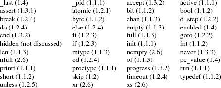
Keywords
For reference, the following table contains all the keywords, predefined functions, predefined variables, and special label-prefixes of the language PROMELA, and refers to the section of this paper in which they were discussed.
References
[Ho91] G.J. Holzmann, Design and Validation of Computer Protocols, Prentice Hall, 1991.
[Ho93] G.J. Holzmann, ‘‘Tutorial: Design and Validation of Protocols,’’ Computer Networks and ISDN Systems, 1993, Vol. 25, No. 9, pp. 981-1017.
[HoPe94] G.J. Holzmann and D.A. Peled, ‘‘An improvement in formal verification,’’ Proc. 7th Int. Conf. on Formal Description Techniques, FORTE94, Berne, Switzerland. October 1994.
[Ho95] G.J. Holzmann, ‘‘An Analysis of Bitstate Hashing,’’ technical report 2/95, available from author.
[HS99] G.J. Holzmann, ‘‘Software model checking: extracting verification models from source code,’’ Proc. Formal Methods in Software Engineering and Distributed Systems, PSTV/FORTE99, Beijng, China, Oct. 1999, Kluwer,pp. 481-497.